Capacity Planning Without a Crystal Ball

Every capacity incident sounds the same in the retrospective. Traffic went up 20%, and latency went up 900%. Nobody deployed anything. The graphs look like a cliff, and the obvious question is why the system did not simply get 20% slower.

The answer is queueing, and it is the one piece of theory in this module worth knowing precisely, because it explains the shape of nearly every performance incident you will ever attend.

Little's Law, and the one formula you need

For any stable system:

L = λ × W
 
L = concurrent requests in the system
λ = arrival rate (requests per second)
W = time each request spends in the system (seconds)

400 requests per second, each taking 250ms, means 100 requests are in flight at any moment, so you need 100 units of concurrency: threads, connections, workers, whatever your runtime calls them.

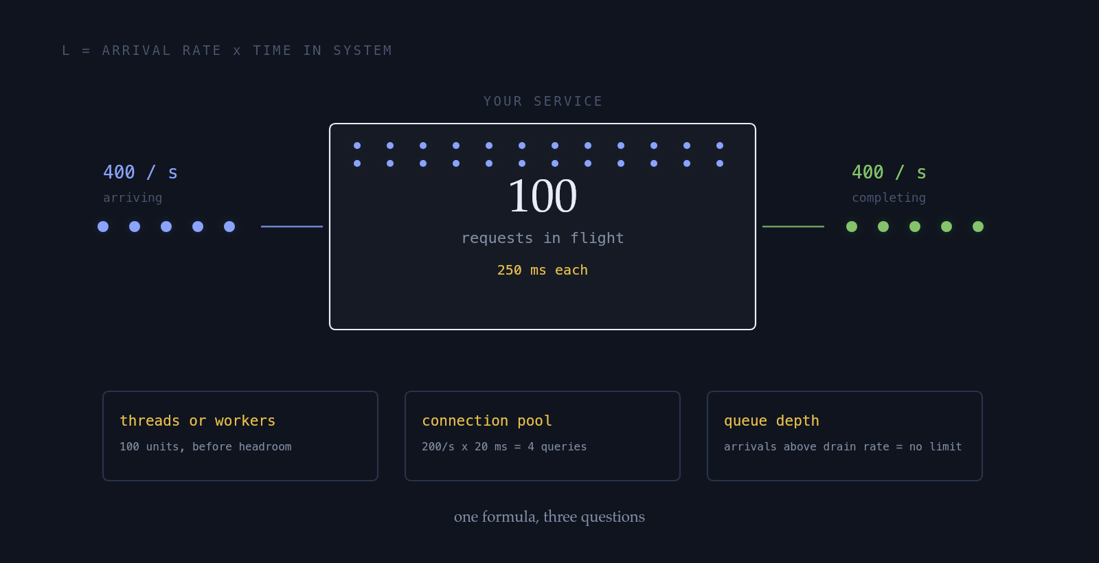
The connection-pool reading is the one that surprises people: 200 QPS with a 20ms query is four concurrent queries, so the right pool size is far smaller than teams guess, and a pool of 100 mostly buys you a queue inside the database. The queue-depth reading is the one that matters at 3am: if arrivals exceed the drain rate, W grows without bound, there is no steady state, and the only question left is where the backlog piles up.

Why latency collapses instead of degrading

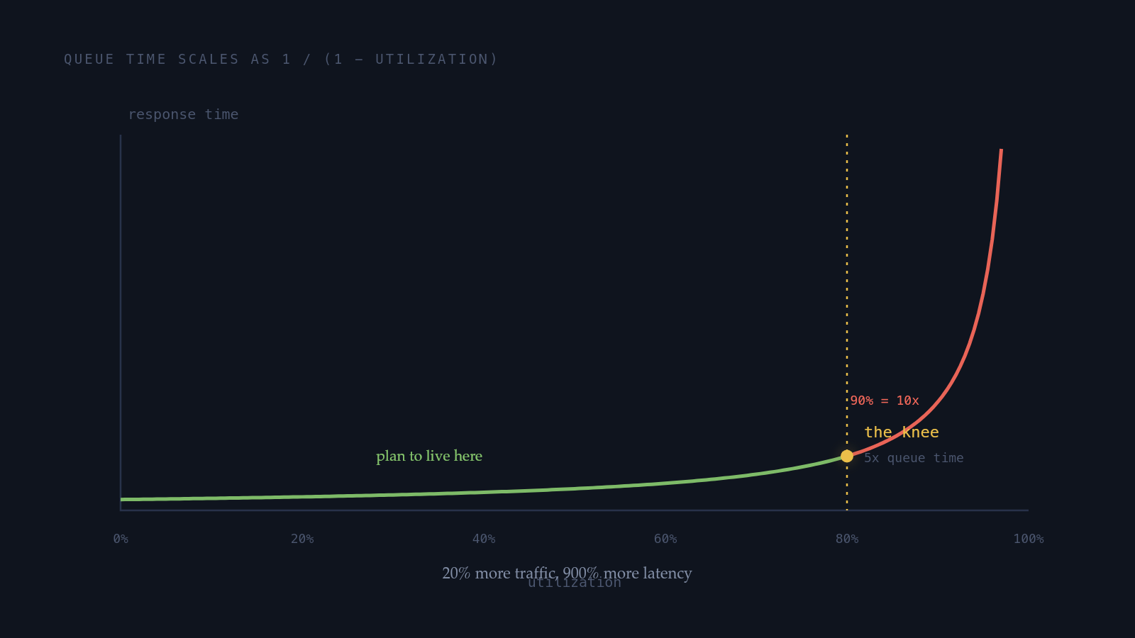
Response time is service time plus queue time. Service time is roughly constant. Queue time depends on utilization, and it does not grow linearly.

For a simple queue, the waiting time scales with 1 / (1 - utilization). That factor is 1.25 at 20% utilization, 2 at 50%, 5 at 80%, 10 at 90%, and 100 at 99%.

Two consequences follow, and they are the whole reason capacity planning exists.

The knee is around 70 to 80%. Below it, extra load is nearly free. Above it, small load increases produce large latency increases, so planning to run at 90% is planning to live on the steep part, where a 5% traffic bump is an incident.

Variability moves the knee left. That formula assumes smooth arrivals and identical work. Real traffic is bursty and a cache hit is not a cache miss, so the more variable the workload, the more headroom the same latency target needs.

This is also why backpressure matters more than capacity. Once you are past the knee, the only options are to shed work or to let the queue grow, and an unbounded queue converts a latency problem into an outage.

How much headroom, and why

"Keep 30% headroom" is a habit, not an answer. The real number comes from asking what you must survive without degrading.

These stack, and the stacking is the part that gets missed. Surviving the loss of one zone during your daily peak means the peak-time load, after losing a third of the fleet, must still land below the knee. That is the design constraint, and it is considerably stricter than the average-utilization number on the dashboard.

Where autoscaling fits: it handles gradual, predictable changes well (the daily cycle) and abrupt ones badly, because instances take minutes to become useful and the spike takes seconds. So autoscaling manages your cost, and static headroom plus load shedding manages your incidents. Treating autoscaling as a spike defense is a common and expensive mistake.

Find the actual bottleneck first

Capacity work aimed at the wrong resource is a rounding error. Brendan Gregg's USE method locates it fastest: per resource, check utilization, saturation, and errors.

Saturation is the one people skip and usually where the answer is. CPU at 60% looks fine until the run queue is 12 deep. Same for a pool that is not "full" but has requests waiting on checkout, and a disk whose throughput is fine while its queue depth is not.

Check in this order, because each one masks the ones after it: thread and connection pools, then the database (usually the real ceiling: find the top query by total time), then CPU, then network and disk. In most request-serving systems the ceiling is a pool limit or the database, not raw compute.

The plan, in five lines

A capacity plan does not need to be a document. It needs these numbers written down somewhere a person will find them during an incident.

1. Current peak QPS, and the peak-to-average ratio.
2. Measured capacity per instance at your latency target, from a load test, not from arithmetic.
3. Required headroom, derived from your failure domain and your peak.
4. The trigger for adding capacity: a utilization or latency threshold, not a feeling.
5. What gets shed first when you exceed all of the above, decided in advance.

Line 5 is the one that separates a plan from a wish. Every system eventually gets more load than it has capacity for, and having already decided which work degrades (search suggestions, recommendation widgets, non-critical writes) is the difference between a slow page and an outage.

Next, the capstone runs every number in this module end to end on one brief: users to QPS, QPS to instances, an SLO, and the headroom to defend it.

Key takeaways

• Little's Law (L = λ × W) sizes pools, workers, and instance counts, and it is the same formula every time.
• Queue time scales as 1/(1 - utilization): 2x at 50% utilization, 5x at 80%, 10x at 90%. That is why latency collapses rather than degrading.
• The knee is at roughly 70 to 80% utilization, and workload variability moves it left. Plan to sit below it.
• Derive headroom from what you must survive (an instance, a zone, the daily peak) and remember those constraints stack.
• Autoscaling controls cost, not spikes. Static headroom plus load shedding controls incidents.
• Find the real bottleneck with utilization, saturation, and errors. Saturation is usually where the answer is, and the database is usually the ceiling.
• Decide in advance what gets shed first. That decision is the plan.