Embeddings Are an Index, Not Magic

Lesson 1 decided that retrieval is the right answer. Underneath it is an index.

A vector index has a build phase, build and query parameters, a size on disk, a memory residency problem, and a correctness knob traded against latency. Every instinct about adding a B-tree to a hot table transfers, with one difference: this index is allowed to be wrong, and you choose how wrong.

An embedding is a coordinate, and the model version owns the space

An embedding is not a summary or a fingerprint. It is a list of floats produced by running text through one model, placing that text at a point in a space that model alone defines. Same input and model version, same vector. A different version returns a valid vector in a different space, not comparable to the first.

The analogue is a hash-partitioned table where someone swapped the hash function: nothing is corrupt, every stored value is a correct answer to a question you stopped asking. Distances across two model versions are meaningless rather than merely worse, and nothing errors.

So the discipline is the one module 2 applied to the generation model: pin the exact embedding model ID and store it beside the vector. A model column tells you which rows live in which space: the difference between an incremental migration and a truncate. Changing the model means re-embedding the corpus, and the ingestion pipeline lesson owns that backfill.

Dimension counts come from the model: text-embedding-3-small emits 1536, text-embedding-3-large 3072, the voyage-4 family defaults to 1024, Cohere's embed-v4.0 to 1536. Retrieval models also need to know whether text is query or document (Voyage's input_type of "query" or "document", Cohere's search_query or search_document). Embedding queries as documents is a silent quality regression: no error, just worse ranking.

The distance metric is a documentation lookup, not a preference

Three metrics dominate (cosine, inner product, and L2), and which one you use is decided by your embedding provider's documentation. Cosine measures the angle and ignores magnitude, inner product is the raw dot product, L2 is straight-line distance.

For vectors normalized to length 1, all three produce identical rankings. OpenAI and Voyage state their vectors are unit length, and pgvector's README picks for you: "If vectors are normalized to length 1 (like OpenAI embeddings), use inner product for best performance."

That equivalence is a consequence of normalization, not a general law. Cohere's docs use cosine in examples but make no explicit unit-norm claim, so do not assume one.

pgvector hides a trap in the syntax: <#> returns the negative inner product, because Postgres only supports ascending index scans. Ordering by it ascending gives most-similar-first; as a displayed score it needs multiplying by -1.

-- Normalized vectors: same ranking as cosine, cheaper per comparison.
CREATE INDEX ON doc_chunks USING hnsw (embedding vector_ip_ops);
 
-- <#> is the NEGATIVE inner product, so plain ASC is "closest first".
SELECT id, (embedding <#> $1) * -1 AS inner_product
FROM doc_chunks
ORDER BY embedding <#> $1
LIMIT 10;

Approximate nearest neighbour is an index with a recall knob

Exact nearest-neighbour search is a sequential scan: compare the query against every row, sort, take k. Recall is 100 percent and cost grows linearly with rows. An approximate index buys sublinear query time by agreeing to miss some results, and every parameter it exposes moves that trade.

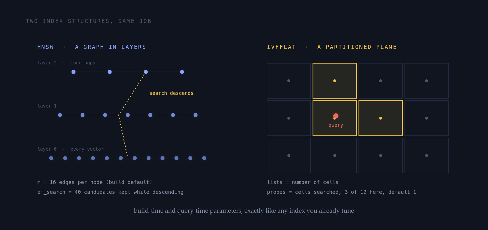
pgvector ships exactly two index types. HNSW is a layered proximity graph from Malkov and Yashunin's 2016 paper: long hops on sparse upper layers reach the right neighbourhood, short hops at the bottom refine. Build it with m (max connections per layer, default 16) and ef_construction (build-time candidate list, default 64); query it with hnsw.ef_search, default 40. IVFFlat instead partitions vectors into lists around centroids and searches the nearest few, via ivfflat.probes, default 1.

Both are session settings: SET LOCAL in a transaction scopes them to one statement. An IVFFlat index left at one probe will convince you vector search does not work.

Recall is a number you measure on your own corpus

Vendor recall figures come from public benchmark datasets. Yours has to be measured on your data, against a brute-force ground truth. Take a sample of real queries from your logs, run each as an exact scan for the true top-k, run them through the index, and average the overlap.

// recall@k: mean overlap between index results and exact-scan ground truth.
export function recallAtK(exact: string[][], approx: string[][], k: number): number {
  let hits = 0;
  let denom = 0;
  for (let i = 0; i < exact.length; i++) {
    const truth = new Set(exact[i].slice(0, k));
    hits += approx[i].slice(0, k).filter((id) => truth.has(id)).length;
    denom += Math.min(k, exact[i].length);
  }
  return hits / denom;
}

One warning about the name. This recall asks how much of the exact answer set the index found, and it is the only recall you can compute without labels. The recall you will gate CI on asks how many human-labelled relevant chunks reached the top k, and the eval guide owns that one. Same word, different measurement.

Run that once per candidate setting and you get a curve, not an opinion: recall climbs steeply while latency barely moves, then flattens while latency climbs. The knee is your operating point, and it belongs to your corpus.

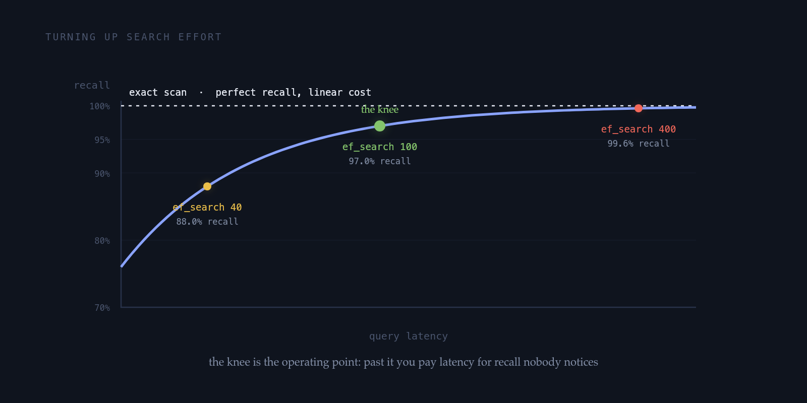
On a small corpus, exact scan is a legitimate production choice: no tuning, perfect recall. The same ef_search bound is why a filtered query can return fewer rows than its LIMIT, and recall is not answer quality either: a retriever at 98 percent recall over badly chosen chunks still answers badly. Retrieval quality handles both, and ships the SQL for the filtered case.

What a dimension costs

Dimension count is a storage, memory, and index-size decision, and the ceiling that bites is the index limit, not the column limit. In pgvector a vector occupies 4 * dimensions + 8 bytes: 6,152 bytes per row at 1536 dimensions, roughly 6 GB per million rows before the HNSW graph exists, 12 GB at 3072. Since HNSW query speed needs the graph resident, this is a RAM budget wearing a disk-space costume.

The limit that surprises everyone: a vector column holds 16,000 dimensions, but an HNSW or IVFFlat index on one caps at 2,000, so text-embedding-3-large's 3072 dimensions are storable and not indexable. The documented escape hatches are halfvec (2 * dimensions + 8 bytes, indexable to 4,000), an expression index over binary_quantize(embedding)::bit(N) with bit_hamming_ops (indexable to 64,000, a cheap first pass re-ranked by exact distance), or indexing a subvector.

The cheaper move is to ask for fewer dimensions at the source. OpenAI's dimensions parameter works only on text-embedding-3 and later, so it cannot shorten ada-002. Voyage's output_dimension offers 256, 512, 1024 and 2048, plus an output_dtype of int8 or binary for 4x and 32x size cuts; Cohere's embed-v4.0 offers 256, 512, 1024 and 1536.

Key takeaways

• An embedding is a coordinate in a space defined by one model version; vectors from two versions give meaningless distances, not errors.
• Pin the embedding model ID beside the vector. A model change is a full re-embed and backfill, not an in-place upgrade.
• Take the distance metric from the provider's docs. For unit-normalized vectors cosine, inner product and L2 rank identically; pgvector recommends vector_ip_ops, and <#> returns the negative inner product.
• HNSW and IVFFlat are pgvector's only index types. The knobs are m, ef_construction and hnsw.ef_search (default 40), and lists and ivfflat.probes (default 1).
• Recall is measured, not inherited: real queries against a brute-force ground truth, recall plotted against latency, operating point at the knee.
• A vector column stores 16,000 dimensions but indexes only 2,000. Use halfvec, binary quantization, or a smaller output dimension, and re-normalize if you truncate by hand.